Selection of guesses
The task described in the discourse discussion mentioned in the previous tutorial was to determine an optimal first guess in Wordle, using the criterion of minimizing the expected pool size after the guess is scored.
First attach the packages that will be used
begin
    using CairoMakie      # graphics package
    using Chain           # sophisticated pipes
    using DataFrameMacros # convenient syntax for df operations
    using DataFrames
    using PlutoUI         # User Interface components
    using Primes          # prime numbers
    using Random          # random number generation
    using StatsBase       # basic statistical summaries
    using Wordlegames
end
In the Wordle game shown on the Wikipedia page the first guess is "arise".
PlutoUI.Resource(
    "https://upload.wikimedia.org/wikipedia/commons/thumb/e/ec/Wordle_196_example.svg/440px-Wordle_196_example.svg.png",
)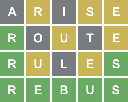
Before the guess is scored the size of the target pool is 2315. The score for this guess in this game is 01011 as a base-3 number or 31 as a decimal number. Of all the targets in the target pool, only 20 will return this score.
To verify this, first create a GamePool from the wordle targets.
begin
    datadir = joinpath(pkgdir(Wordlegames), "data")
    wordle = GamePool(collect(readlines(joinpath(datadir, "Wordletargets.txt"))))
end;
Then determine the index of "arise" in the guess pool.
only(findall(x -> x == ('a', 'r', 'i', 's', 'e'), wordle.guesspool))106Here, findall returns a vector of all positions in wordle.guesspool that return true from the anonymous function checking if the argument, x, is equal to ('a', 'r', 'i', 's', 'e'). The only function checks that there is only one such index and, if so, returns it.
The anonymous function to compare an element of wordle.guesspool to ('a','r','i','s','e') can be written more compactly as ==(('a','r','i','s','e')).
The score for the guess "arise" on the target "rebus" is 31 as a decimal number.
Int(wordle.allscores[only(findall(==(('r', 'e', 'b', 'u', 's')), wordle.guesspool)), 106])31Next, check how many of the pre-computed scores in the 106th column of wordle.allscores are equal to 31.
sum(==(31), view(wordle.allscores, :, 106))20A view provides access to a subarray of an array without copying the contents. In this case the subarray is all the rows (the : argument in the rows position) and the 106th column. The comparison function ==(31) will return true or false, values that will be converted for 1 or 0 for the summation function sum. Thus sum(==(31), v) returns the number of elements of v that are equal to 31.
The distribution of scores for a guess
In this case the first guess reduced the size of the target pool from 2315 to 20, after this guess was scored. Ideally we want a guess to reduce the size of the target pool as much as possible but we don't know what the score is going to be. However, we can evaluate the distribution of pool sizes that will result from a particular guess.
To do this we "bin" the scores for a guess on the active targets into the 243 possible values for an NTuple{5,Char}.
bincounts!(wordle, 106).counts243-element Vector{Int64}:
168
121
61
80
41
17
17
⋮
0
0
0
0
0
1The i'th element of this vector is the number of targets that will give a score of i - 1 for guess = wordle.guesspool[106], which is "arise"
The most common score is 0 which is returned for 168 of the 2315 targets currently in the target pool.
sum(iszero, view(wordle.allscores, :, 106))168Collecting the bin sizes and the corresponding scores in a data frame allows us to sort them by decreasing count size and eliminate the scores that give counts of zero.
df106 = @chain DataFrame(score=tiles.(0:242, 5), counts=wordle.counts) begin
    @subset(:counts > 0)
    sort(:counts; rev=true)
end| score | counts |
|---|---|
| "🟫🟫🟫🟫🟫" | 168 |
| "🟨🟫🟫🟫🟫" | 154 |
| "🟫🟫🟫🟫🟨" | 121 |
| "🟫🟫🟨🟫🟫" | 107 |
| "🟫🟨🟫🟫🟨" | 100 |
| "🟫🟫🟫🟨🟫" | 80 |
| "🟨🟫🟫🟫🟨" | 79 |
| "🟫🟨🟫🟫🟫" | 64 |
| "🟨🟨🟫🟫🟫" | 62 |
| "🟫🟫🟫🟫🟩" | 61 |
| ... | |
| "🟩🟩🟩🟩🟩" | 1 |
A bar plot of the bin sizes, ordered from largest to smallest is
barplot(df106.counts)
The Wordlegames package provides two algorithms of choosing a guess based on the distribution of the scores.
function optimalguess(gp::GamePool{N,S,MaximizeEntropy}) where {N,S}
    gind, xpctd, entrpy = 0, Inf, -Inf
    for (k, a) in enumerate(gp.active)
        if a
            thisentropy = entropy2(bincounts!(gp, k))
            if thisentropy > entrpy
                gind, xpctd, entrpy = k, expectedpoolsize(gp), thisentropy
            end
        end
    end
    return gind, xpctd, entrpy
end

function optimalguess(gp::GamePool{N,S,MinimizeExpected}) where {N,S}
    gind, xpctd, entrpy = 0, Inf, -Inf
    for (k, a) in enumerate(gp.active)
        if a
            thisexpected = expectedpoolsize(bincounts!(gp, k))
            if thisexpected < xpctd
                gind, xpctd, entrpy = k, thisexpected, entropy2(gp)
            end
        end
    end
    return gind, xpctd, entrpy
end
The first method is to maximize the entropy of the distribution, which is an information-theory concept that measures how "spread out" the distribution is. It depends only on the probabilities of the scores, not on the scores themselves. The base-2 entropy, measured in bits, of a discrete distribution with probabilities $p_i, i=1,\dots,n$ is defined as
$$H_2(X) = - \sum_{i=1}^n p_i\,\log_2(p_i)$$
The Wordlegames package exports the entropy2 function that returns this quantity from the current counts.
function entropy2(counts::AbstractVector{<:Real})
    countsum = sum(counts)
    return -sum(counts) do k
        x = k / countsum
        xlogx = x * log(x)
        iszero(x) ? zero(xlogx) : xlogx
    end / log(2)
end

entropy2(gp::GamePool) = entropy2(gp.counts)entropy2(wordle.counts)5.820939700886001or, equivalently
entropy2(bincounts!(wordle, 106))5.820939700886001The
... do k
   ...
end
block, called a "thunk", in this code - yet another way of writing an anonymous function - is described later.
Roughly, the numerical result means that the distribution of target pool sizes after an initial guess of "arise" is, according to this measure, about as spread out as a uniform distribution on 56.5 possible responses.
2^(entropy2(wordle))56.529800516800876The second method is to minimize the expected pool size after the guess is scored.
By definition this is the sum of the bin size (or count) for each of the bins multiplied by the probability of the target being in the bin. But that probability is the bin size divided by the total number of active targets. Thus the expected pool size after the guess can be evaluated from the bin sizes alone.
function expectedpoolsize(gp::GamePool)
    return sum(abs2, gp.counts) / sum(gp.counts)
end
sum(abs2, wordle.counts) / sum(wordle.counts) # abs2(x) returns x * x 63.72570194384449which is available as expectedpoolsize
expectedpoolsize(bincounts!(wordle, 106))63.72570194384449This is a measure of how successful an initial guess of "arise" will be. On average it will reduce the target pool size from 2315 to 63.73.
The best initial guess?
We can choose an initial guess (and, also, subsequent guesses) to maximize the entropy of the distribution of scores or to minimize the expected pool size for the next guess.
For both of these criteria, a slight modification on "arise", exchanging the first two letters to form "raise", at index 1535, is a bit better than "arise".
string(wordle.guesspool[1535]...)"raise"entropy2(bincounts!(wordle, 1535))5.877909690821478expectedpoolsize(wordle)61.00086393088553It turns out that "raise" is the best initial guess for both of these criteria, if we restrict outselves to guesses from the initial target pool.
One of the parameters of the GamePool type is the method of choosing the next guess, either MaximizeEntropy, the default, or MinimizeExpected,
typeof(wordle)GamePool{5, UInt8, MaximizeEntropy}allowing for automatic game play.
showgame!(wordle, "rebus")| poolsz | index | guess | expected | entropy | score | sc |
|---|---|---|---|---|---|---|
| 2315 | 1535 | "raise" | 61.0009 | 5.87791 | "🟩🟫🟫🟨🟨" | 166 |
| 2 | 1558 | "rebus" | 1.0 | 1.0 | "🟩🟩🟩🟩🟩" | 242 |
That game ended suspiciously quickly but notice that, after the first guess, "raise", is scored as 🟩🟫🟫🟨🟨 in tiles or 166 in decimal, the target pool size is reduced to 2,
[string(wordle.targetpool[i]...) for i in findall(==(166), view(wordle.allscores, :, 1535))]2-element Vector{String}:
"rebus"
"reset"giving a 50% chance of a correct second guess.
In the case of ties like this the target with the lowest index in the targetpool is returned. This strategy can result in long series of guesses trying to isolate a single letter if that letter is toward the end of the alphabet
showgame!(wordle, "watch")| poolsz | index | guess | expected | entropy | score | sc |
|---|---|---|---|---|---|---|
| 2315 | 1535 | "raise" | 61.0009 | 5.87791 | "🟫🟩🟫🟫🟫" | 54 |
| 91 | 2012 | "tangy" | 7.48352 | 4.03061 | "🟨🟩🟫🟫🟫" | 135 |
| 13 | 334 | "caput" | 2.84615 | 2.4997 | "🟨🟩🟫🟫🟨" | 136 |
| 5 | 160 | "batch" | 3.4 | 0.721928 | "🟫🟩🟩🟩🟩" | 80 |
| 4 | 959 | "hatch" | 2.5 | 0.811278 | "🟫🟩🟩🟩🟩" | 80 |
| 3 | 1102 | "latch" | 1.66667 | 0.918296 | "🟫🟩🟩🟩🟩" | 80 |
| 2 | 1206 | "match" | 1.0 | 1.0 | "🟫🟩🟩🟩🟩" | 80 |
| 1 | 2233 | "watch" | 1.0 | -0.0 | "🟩🟩🟩🟩🟩" | 242 |
but it is not clear that any other strategy will be more successful across all possible targets. (This target did occur on the official Wordle web site in March of 2022.)
To play by the MinimizeExpected strategy requires specifying this as the guesstype when creating the GamePool.
wordlexpct = GamePool(
    collect(readlines(joinpath(datadir, "Wordletargets.txt")));
    guesstype=MinimizeExpected,
);
showgame!(wordlexpct, "rebus")| poolsz | index | guess | expected | entropy | score | sc |
|---|---|---|---|---|---|---|
| 2315 | 1535 | "raise" | 61.0009 | 5.87791 | "🟩🟫🟫🟨🟨" | 166 |
| 2 | 1558 | "rebus" | 1.0 | 1.0 | "🟩🟩🟩🟩🟩" | 242 |
showgame!(wordlexpct, "watch")| poolsz | index | guess | expected | entropy | score | sc |
|---|---|---|---|---|---|---|
| 2315 | 1535 | "raise" | 61.0009 | 5.87791 | "🟫🟩🟫🟫🟫" | 54 |
| 91 | 2012 | "tangy" | 7.48352 | 4.03061 | "🟨🟩🟫🟫🟫" | 135 |
| 13 | 334 | "caput" | 2.84615 | 2.4997 | "🟨🟩🟫🟫🟨" | 136 |
| 5 | 160 | "batch" | 3.4 | 0.721928 | "🟫🟩🟩🟩🟩" | 80 |
| 4 | 959 | "hatch" | 2.5 | 0.811278 | "🟫🟩🟩🟩🟩" | 80 |
| 3 | 1102 | "latch" | 1.66667 | 0.918296 | "🟫🟩🟩🟩🟩" | 80 |
| 2 | 1206 | "match" | 1.0 | 1.0 | "🟫🟩🟩🟩🟩" | 80 |
| 1 | 2233 | "watch" | 1.0 | -0.0 | "🟩🟩🟩🟩🟩" | 242 |
There are no differences between the two strategies in these games.
However, if we play all possible games using each of the two strategies and count the number of guesses to solution we can see that the two strategies do not always give the same length of game.
gamelen = let
    inds = axes(wordle.targetpool, 1)
    DataFrame(;
        index=inds,
        entropy=[length(playgame!(wordle, k).guesses) for k in inds],
        expected=[length(playgame!(wordlexpct, k).guesses) for k in inds],
    )
end| index | entropy | expected |
|---|---|---|
| 1 | 3 | 3 |
| 2 | 3 | 3 |
| 3 | 3 | 3 |
| 4 | 4 | 4 |
| 5 | 3 | 4 |
| 6 | 4 | 3 |
| 7 | 3 | 3 |
| 8 | 4 | 4 |
| 9 | 3 | 3 |
| 10 | 3 | 3 |
| ... | ||
| 2315 | 5 | 4 |
For example,
showgame!(wordle, 5)| poolsz | index | guess | expected | entropy | score | sc |
|---|---|---|---|---|---|---|
| 2315 | 1535 | "raise" | 61.0009 | 5.87791 | "🟫🟨🟫🟫🟫" | 27 |
| 92 | 766 | "float" | 4.54348 | 4.86323 | "🟫🟫🟨🟨🟩" | 14 |
| 1 | 5 | "abbot" | 1.0 | -0.0 | "🟩🟩🟩🟩🟩" | 242 |
is different from
showgame!(wordlexpct, 5)| poolsz | index | guess | expected | entropy | score | sc |
|---|---|---|---|---|---|---|
| 2315 | 1535 | "raise" | 61.0009 | 5.87791 | "🟫🟨🟫🟫🟫" | 27 |
| 92 | 414 | "cloak" | 4.17391 | 4.64926 | "🟫🟫🟨🟨🟫" | 12 |
| 5 | 88 | "annoy" | 1.0 | 2.32193 | "🟩🟫🟫🟩🟫" | 168 |
| 1 | 5 | "abbot" | 1.0 | -0.0 | "🟩🟩🟩🟩🟩" | 242 |
The mean and standard deviation of the game lengths are smaller when maximizing the entropy than when minimizing the expected pool size.
describe(gamelen[!, [:entropy, :expected]], :min, :max, :mean, :std)| variable | min | max | mean | std |
|---|---|---|---|---|
| :entropy | 1 | 8 | 3.59914 | 0.849016 |
| :expected | 1 | 8 | 3.62462 | 0.857827 |
The counts of the game lengths under the two strategies and a comparative barplot show the shift toward shorter game lengths when maximizing the entropy.
gamelengths = let
    entropy = countmap(gamelen.entropy)
    expected = countmap(gamelen.expected)
    allcounts = 1:maximum(union(keys(entropy), keys(expected)))
    DataFrame(;
        count=allcounts,
        entropy=[get!(entropy, k, 0) for k in allcounts],
        expected=[get!(expected, k, 0) for k in allcounts],
    )
end| count | entropy | expected |
|---|---|---|
| 1 | 1 | 1 |
| 2 | 131 | 131 |
| 3 | 999 | 957 |
| 4 | 919 | 946 |
| 5 | 207 | 224 |
| 6 | 47 | 42 |
| 7 | 9 | 11 |
| 8 | 2 | 3 |
let
    stacked = stack(gamelengths, 2:3)
    typeint = [(v == "entropy" ? 1 : 2) for v in stacked.variable]
    barplot(
        stacked.count,
        stacked.value;
        dodge=typeint,
        color=typeint,
        axis=(xticks=1:8, xlabel="Game length", ylabel="Number of targets"),
    )
end
Wordle-like games
Wordle has spawned many similar games, one of which is Primel, where the targets are 5-digit prime numbers. Because leading zeros are not allowed in these primes, the targets are prime numbers between 10,000 and 99,999.
primel = GamePool(primes(10_000, 99_999)); # underscores are ignored in numbersTo play a game with a random, but reproducible, target, we initialize a random number generator and pass it as the second argument to showgame!.
showgame!(primel, Random.seed!(1234321))| poolsz | index | guess | expected | entropy | score | sc |
|---|---|---|---|---|---|---|
| 8363 | 313 | "12953" | 124.384 | 6.63227 | "🟨🟨🟫🟫🟫" | 108 |
| 201 | 1141 | "21067" | 5.92537 | 5.47937 | "🟨🟨🟫🟨🟨" | 112 |
| 10 | 3556 | "46271" | 1.2 | 3.12193 | "🟩🟩🟩🟩🟩" | 242 |
The size of the target pool is larger than for Wordle
length(primel.targetpool)8363but the number of possible characters at each position (9 for the first position, 10 for the others) is smaller than for Wordle, leading to a larger mean number of guesses but a smaller standard deviation in the number of guesses.
As for Wordle, the strategy of choosing guesses to minimize the expected pool size is less effective than maximizing the entropy.
primelxpectd = GamePool(primes(10_000, 99_999); guesstype=MinimizeExpected);allprimel = let
inds = 1:length(primel.targetpool)
DataFrame(;
index=inds,
entropy=[length(playgame!(primel, k).guesses) for k in inds],
expected=[length(playgame!(primelxpectd, k).guesses) for k in inds],
)
end| index | entropy | expected |
|---|---|---|
| 1 | 4 | 4 |
| 2 | 4 | 4 |
| 3 | 3 | 4 |
| 4 | 3 | 4 |
| 5 | 3 | 4 |
| 6 | 3 | 3 |
| 7 | 4 | 4 |
| 8 | 4 | 4 |
| 9 | 4 | 4 |
| 10 | 3 | 4 |
| ... | ||
| 8363 | 5 | 4 |
primelengths = let
    entropy = countmap(allprimel.entropy)
    expected = countmap(allprimel.expected)
    allcounts = 1:maximum(union(keys(entropy), keys(expected)))
    DataFrame(;
        count=allcounts,
        entropy=[get!(entropy, k, 0) for k in allcounts],
        expected=[get!(expected, k, 0) for k in allcounts],
    )
end| count | entropy | expected |
|---|---|---|
| 1 | 1 | 1 |
| 2 | 215 | 209 |
| 3 | 3173 | 2743 |
| 4 | 4477 | 4797 |
| 5 | 482 | 589 |
| 6 | 15 | 24 |
describe(allprimel[!, Not(1)], :min, :max, :mean, :std)| variable | min | max | mean | std |
|---|---|---|---|---|
| :entropy | 1 | 6 | 3.63004 | 0.641331 |
| :expected | 1 | 6 | 3.69784 | 0.647833 |
let
    stacked = stack(primelengths, 2:3)
    typeint = [(v == "entropy" ? 1 : 2) for v in stacked.variable]
    barplot(
        stacked.count,
        stacked.value;
        dodge=typeint,
        color=typeint,
        axis=(xticks=1:8, xlabel="Game length", ylabel="Number of targets"),
    )
end
Some Julia syntax used in this code
Several Julia syntax features have been used in the code for this tutorial. For example, the code block defining gamelengths is a let block. This is similar to a begin/end block in that it groups multiple expressions, including assignments, so that they function as a single expression evaluation. The difference between let and begin is that assignments within a let block are local to the block.
For example, allcounts is given a value within that block because it is used in several places when creating the DataFrame but it is not needed outside that block.
Notice also the expressions like get!(entropy, k, 0). This is extraction by key from a collection, like entropy[k] or, equivalently, getindex(entropy, k) except that it provides a default, 0 in this case, if there is no key k in the collection. Furthermore, it modifies the collection by inserting the default value for key k.
An ellipsis, "...", is used with arguments as in string(wordle.guesspool[1535]...). This use is called a "splat" (and there is another use of an ellipsis called a "slurp" - the designers of this language are very serious-minded folk). As a "splat" the ellipsis expands an argument such as a vector or, in this case, the tuple ('r','a','i','s','e') to multiple arguments, in this case, 5 Char arguments.
Another fun name for a construct is a "thunk", which is a way of specifying an anonymous function. For example there are two methods defined for the entropy2 generic
function entropy2(counts::AbstractVector{<:Real})
    countsum = sum(counts)
    return -sum(counts) do k
        x = k / countsum
        xlogx = x * log(x)
        iszero(x) ? zero(xlogx) : xlogx
    end / log(2)
end

entropy2(gp::GamePool) = entropy2(gp.counts)
In the first method we wish to evaluate $-\sum_{i}p_i\,\log_2(p_i)$ which is sometimes called an xlogx function. There is a sum(f, itr) method where f is a function and itr is an iterator, such as an AbstractVector. In this case we want a function that evaluates x = k / countsum then xlogx(x) but xlogx requires some care. If x is zero, the result should be zero but of the same type as x * log(x) for non-zero x. That's why x * log(x) is evaluated first - to get the value type. It will return NaN for x = 0, which is then converted to a zero but of the type that is consistent with the other values of xlogx.
For example, to evaluate the base-2 entropy for the initial guess in the BigFloat extended precision type, we convert from
bincounts!(reset!(wordle), 1535); # reset the game to the initial stateentropy2(wordle.counts)5.877909690821478to
entropy2(big.(wordle.counts))5.877909690821480658631076345837703704414854243834085634605204301304453462519103The second method definition for entropy2 shows the compact form for defining "one-liner" methods. It is a common idiom to have one method for a generic function that "does the work" and others that simply re-arrange the arguments to the form required by this "collector" method.
Built with Julia 1.7.2 and
CairoMakie 0.7.5Chain 0.4.10
DataFrameMacros 0.2.1
DataFrames 1.3.2
PlutoUI 0.7.38
Primes 0.5.2
StatsBase 0.33.16
Wordlegames 0.3.0
To run this tutorial locally, download this file and open it with Pluto.jl.